Climate imperative: lower natural gas

Tractor swarm Dover Plains NY January 2019
Qualitative summary Earth’s atmosphere handles methane and CO2 very differently. It disposes completely (mostly by oxidation) of an inflow of methane within about ten years, but constantly renews its stock of CO2 through the carbon cycle. So, where CO2 emissions must always add to atmospheric heat-trapping and thus to global heating, methane emissions need not. If annual methane emissions are just kept level year over year for a decade, their addition to heat-trapping will be ZERO. A steady decline in annual emissions over that period will allow cooling, where even a steep drop in CO2 emissions won’t.
The Global Warming Potential that compares methane to CO2 hides that crucial difference: humanity has leverage over methane’s future additions to heat-trapping that we don’t with additions by CO2. As we strive to lower CO2 emissions, we must exert our leverage on methane by halting the annual growth of [mostly fracked] natural gas production, now the chief driver of human-influenced methane emissions. To end that growth demands an abrupt cutoff of all new natural gas infrastructure. Cricket Valley Energy, CPV Valley, Danskammer, National Grid E37 Albany Loop and the Williams pipeline under NY Harbor (to name just five) must all be stopped in their tracks. This is a climate imperative.
Quantitative summary Suppose methane emissions in 2029 = 351 million metric tons (Mmt). How much heat-trapping capacity will that add to the atmosphere? Using GWP20 (global warming potential) of 86, the equivalent of 30 Gt (gigatons or billion metric tons) of CO2, almost as much as the 37 Gt of actual CO2 emissions in 2018. THIS CLIMATE DEATH BLOW CAN BE AVERTED BY ACTION STARTING NOW. Here’s why:
The atmosphere disposes of a year’s inflow of methane (mostly by oxidation) within about ten years, but constantly replenishes its stock of CO2 through the carbon cycle. If methane emissions over the next ten years never exceed 351 Mmt/yr , that mass released in 2029 will add to the atmosphere the heating-up equivalent of ZERO mt of CO2. CO2 emissions always add; methane emissions need not. In fact, steadily falling methane emissions will allow cooling to begin after ten years, where falling CO2 emissions will never.
To keep methane emissions level 2019-2029, natural gas (NG) withdrawal and consumption must be held level; leaks and losses of methane from the NG supply chain are now the main source of human-influenced methane releases. To end all new natural gas infrastructure is a climate imperative. Come 2029, do we want methane to add the heating equivalent of 30 Gt CO2 to the atmosphere or the equivalent of ZERO ? “Therefore, choose life.” Deut 30:19
Cricket Valley Energy, CPV Valley, Danskammer, National Grid E37 Albany Loop and the Williams pipeline under NY Harbor (to name just five) must all be stopped in their tracks.
Introduction There are many good reasons to ban fracking. Not always at the forefront among them is that fracking has led to a tremendous increase since 2006 in the withdrawal and marketing of natural gas (NG), especially in the USA. Total production rose by 62% from 518 bcm in 2006 to 841 bcm in 2018. In that time conventional went down by 58% and unconventional i.e. “fracked” rose by 273%. Graph 1 . The surge in production of NG, which is about 93% methane, causes increased emissions of the super-efficient greenhouse gas methane.
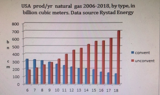
Graph 1. Natural gas production in USA by type (conventional vs. unconventional AKA “fracked”) 2006-2018 in billion cubic meters/yr source Rystad Energy
GWP, (global warming potential) says that a molecule of methane is 25 to 105 times more efficient at trapping heat in the atmosphere than a molecule of CO2. From this fact, most people think that a one-ton emission of methane will always add to atmospheric heat-trapping capacity the equivalent (termed CO2-e) of 25 to 105 tons of CO2 released at the same time.
There, most people are wrong.
In all scenarios where methane emissions year-on-year have been flat (zero slope) or decreasing (negative slope) for about ten years, calculated CO2-e may be billions of tons yet the year’s emissions will add nothing to atmospheric heat-trapping potential, even let it decrease. This is because the atmosphere disposes of a year’s methane inflows entirely over the next ten or so years while instantly replenishing its stock of CO2 for centuries through the carbon cycle.
To have reached ten years hence this zone of no future added heating from stable ongoing emissions will not end our methane crisis. Atmospheric levels will be much higher than today’s. It is, however, a bend in the arc of methane’s contributions to heat-trapping capacity. The curve of CO2’s additions, by contrast, will always rise until emissions are zero. People fighting fossil fuels need to see we have leverage over methane that we don’t have over CO2. We must use it.
To bend the arc by 2030 we must prevent year on year increases of methane emissions starting 2019. What that would require is unclear. I can find no global methane emission figures (which are famously imprecise anyway) for after 2012. Graph 2 shows that yearly emissions recorded were flat 1990 to 2002, then rose steadily to 2012 except in 2008. The average annual increasein those ten years was 5.8 Mmt (million metric tons) about 2% per year. [Emissions of methane are typically recorded in teragrams (Tg) where 1 Tg = 1 Mmt. For familiarity, Mmt will be used for methane instead of Tg.]
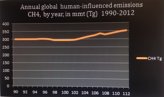
Graph 2. Global human-influenced methane emissions by year 1990-2012 in Tg (million metric tons) Data source EDGAR graph by Shafer
Atmospheric concentrations of methane are more precise and timely than emissions data, though it is hard to relate the two quantitatively. From 2006 to 2018 the concentration rose steadily from 1774 parts per billion (ppb) to 1857 ppb, an average annual increase of about 6 ppb ( + 0.5% of 2006 baseline) (Graph 3, below)
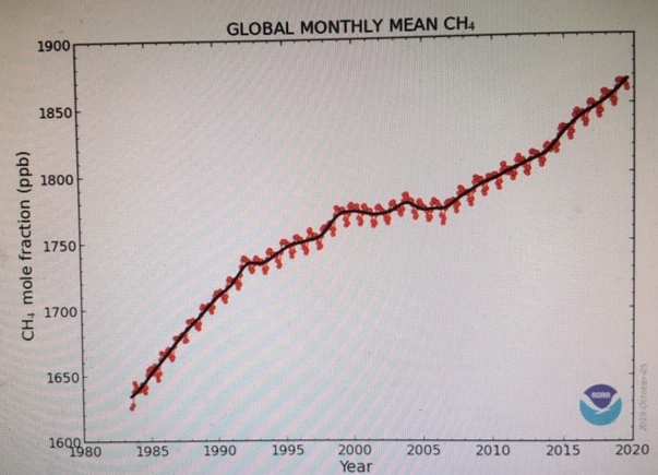
Graph 3. Globally averaged marine surface monthly mean CH4 concentration 1983-2019 Source Ed Dlugokencky NOAA
In short, we don’t know how much annual methane emissions have been changing since 2012. Extrapolation of the 2003-2012 trend and the rise in atmospheric concentrations 2006-2018 indicate they must be going up. How fast, it is impossible to say precisely.
It is plausible, though not proven, that all recent conjectured annual increases in global methane emissions are due to losses of methane from the natural gas supply chain, which moves more gas each year. In 2005 global production of natural gas was 2.8 trillion cubic meters (tcm). By 2018 it had gone up by 1.055 tcm ( + 81 bcm/yr), a 2.9 % average annual increase over baseline. (source Rystad Energy ) [Not incidentally, more than half the increase was from USA “unconventional,” i.e. fracked. (source Rystad Energy )] See Graph 4 below.
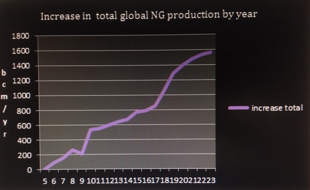
Graph 4. Increase in global total natural gas production above 2005 baseline of 2800 billion cubic meters /yr. Values thru 2018 are real; after that, projected source Rystad Energy
The increase in global supply chain throughput 2017-2018 was 200 bcm; if (say) 5% of that was lost from the chain as methane in that year, the increased emissions would amount to 6.5 Tg or Mmt.. [Arithmetic for that number is in appendix.] Ecological prudence should assume that all the increase in human-influenced methane emissions is due to natural gas withdrawal and distribution; no other emitting sector (e.g. ruminants) is growing at anything like the pace of natural gas. In fact, in the UK at least methane from ruminants is going down. Under this assumption, flattening the curve of natural gas production over the next ten years then holding that course would stop all subsequent additions by methane to atmospheric heating, a sea change. Ending all fossil fuel infrastructure expansion in New York State forwards this strategy. Ending that expansion includes
- No new conventional gas wells; fracked ones are banned
- No new gas pipelines, long or short, no extensions no spurs
- No new or renovated gas-fired power plants
- No new gas storage facilities
- No new buildings hooked up to natural gas
- No exports of liquefied natural gas for fuel or feedstock
- Properly identify and cap all abandoned gas wells
- Carbon fee & dividend on natural gas with agricultural exemption for specified covered fuels
- Top priority for renewable energy sources like wind and solar, battery storage
- Government and private (utility) incentives for renewable heat technologies
- No federal subsidies for natural gas systems
This is not a call to shut down natural gas in the USA in 2020. It is a call to keep it from growing. Cricket Valley Energy, CPV Valley, Danskammer, the proposed National Grid E37 Albany Loop and the proposed Williams pipeline under NY Harbor (to name just five) must all be stopped in their tracks Past that inflection point, withdrawal and consumption need to be reduced speedily in sectors (electricity generation, structure heating) that have a renewable alternative. Reducing methane emissions year on year will start cooling the atmosphere after ten years. Reducing CO2 emissions is crucial, but by itself will never promote cooling.
Supplementary materials:
As said above, the trajectory of methane emissions growth for the last seven years is not known; so, I have simulated five different time trends in annual global human-influenced methane emissions between 2013-2029. These are in Graph 5, below. For all five scenarios, the figures for 2002-2012 are real data derived from the EDGAR (Emissions Data Base for Global Atmospheric Research) data base For all five, figures after 2012 are simulated. The basis of each scenario (A-E) is shown for each scenario in table 1. That table also shows the addition to future atmospheric heating capacity at the end of the simulated time series in 2029 as gauged by four different metrics. CO2-using GWP 100 and using GWP20; CO2-e* (spoken “CO2-e star”) and CO2-we, both of which use the GWP* (spoken “GWP star”) method put forward in several recent publications listed in the references.
For calculation of CO2-e* and CO2-we, refer to my blogs CO2-e is the Wrong Metric and Divergent Metrics
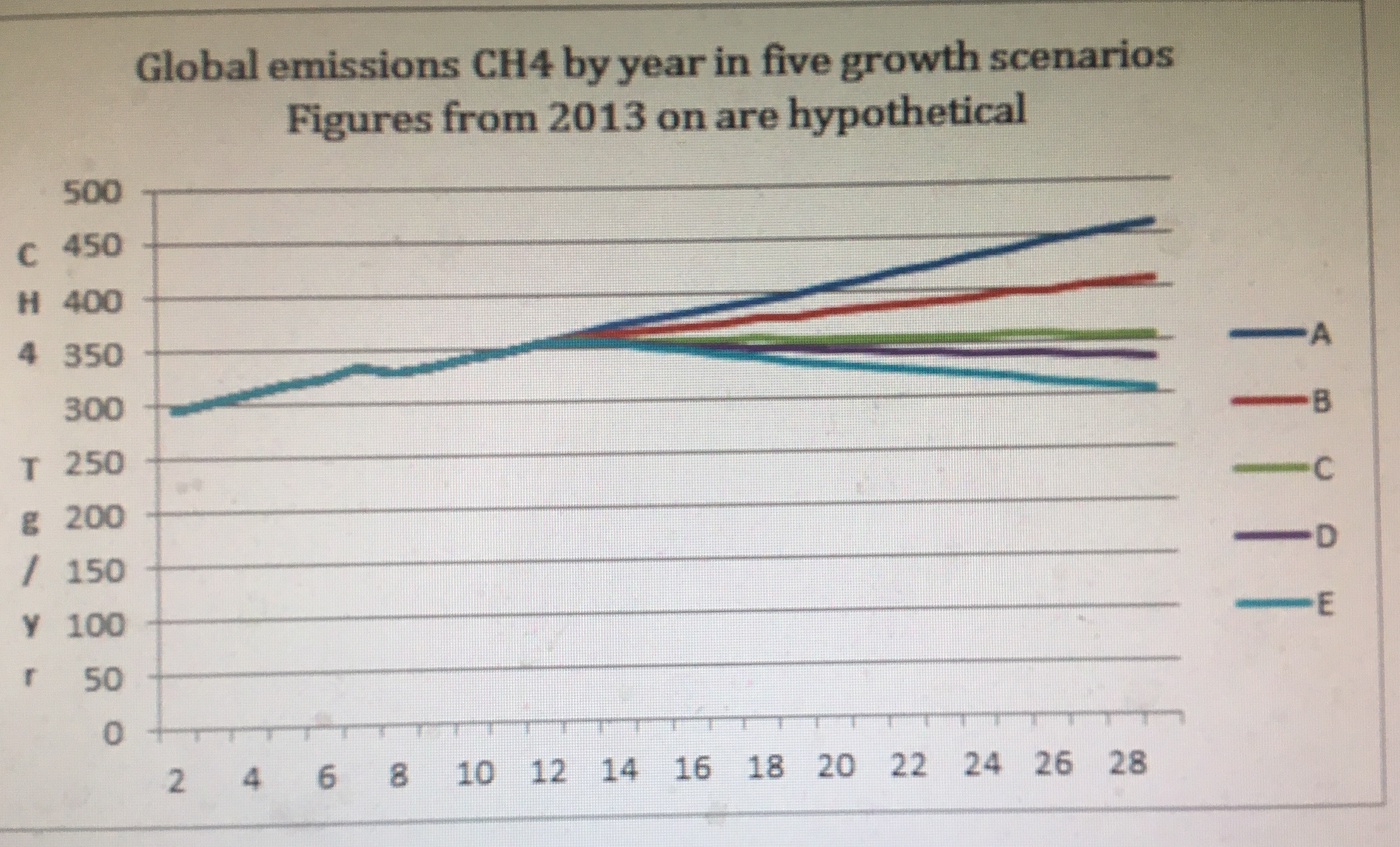
Graph 4. Annual global human-influenced methane emissions in Tg (Mmt), 2002-2029, by growth scenario post-2012 All figures after 2012 are hypothetical for illustrative purposes. Figures for 2002-2012 are derived from EDGAR data base. Horizontal axis is years 2002- 2029 For scenarios A-E see text.
|
A |
B |
C |
D |
E |
F |
G |
H |
|
Scen |
E2012 |
E2029 |
delta E |
CO2-e 100 |
CO2-e* |
CO2-we |
CO2-e 20 |
|
A |
356 |
461 |
105 |
12908 |
17294 |
15470 |
39646 |
|
B |
356 |
403 |
52 |
11,284 |
8564 |
8916 |
34658 |
|
C |
356 |
356 |
0 |
9968 |
0 |
2492 |
30616 |
|
D |
356 |
335.84 |
-20.16 |
9403 |
-3294 |
0 |
28882 |
|
E |
356 |
304 |
-52 |
8512 |
-8564 |
-3920 |
26144 |
Table1 Results of simulated data on global human-influenced methane emissions in millions of metric tons in five hypothetical scenarios for four comparative metrics
Columns in Table 1 are as follows:
A Scenario
B global human-influenced methane emissions in Tg (= Mmt) per year 2012 (real datum)
C global human-influenced methane emissions in Tg (= Mmt) per year 2029 (HYPOTHETICAL)
D interval change of hypothetical annual global human-influenced methane emissions in Tg (= Mmt) 2012-2029
E CO2-e in Mmt per year for 2029 methane emissions using GWP100 of 28
F CO2-e* in Mmt per year for 2029 methane emissions using GWP* methods (Allen, Shine, Fuglestvedt et al 2018)
G CO2-we (warming equivalent ) in Mmt per year for 2029 methane emissions using improved GWP* methods (Cain, Lynch Allen et al 2019)
H CO2-e in Mmt per year for 2029 emissions using GWP20 of 86
Rows (scenario designation)
A Annual increase 2013-2029 follows trend of 2002-2012, averages + 6 Mmt/yr
B Annual increase 2013-2029 lower than in A, averages + 3 Tg/yr
C No increase 2013-2029 , averages 0
D Very small decrease 2013-2029, averages -1.19 Tg/yr
E Small decrease 2013-2029 averages -3 Tg/yr
Observations from Table 1. In scenario A (swift increase in emissions avg 1.7%.yr), CO2-e* and CO2-we are both higher than CO2-e100 and lower than CO2-e20. In B ( increase avg 0.85%/yr) both are lower, because the heat-trapping effect of newly-arrived molecules of the short-lived gas methane is partly offset by disappearance (mostly through oxidation) of earlier arrivals. There is no such offset with CO2 in the bottomless carbon cycle.
Scenario C (avg increase zero/yr) is the centerpiece. CO2-e from either GWP horizon. (20 or 100 years) are both in billions of metric tons while CO2-e* is nil. If this scenario held constant after 2029, there would be no addition to radiative forcing by methane after that year. By then, however, there would have been a considerable, very damaging buildup that would be sustained by level emissions. CO2-we, as in all scenarios of slight positive slope or no slope or negative slope, has a higher value than CO2-e* . Here CO2-we is 2,492, higher than zero for CO2-e* but much lower than the CO2-e of 9968 M mt. Why CO2-we is higher that CO2-e* is explained in Cain, Lynch. Allen et al (2019)
Scenario D (small decrease averaging 0.33% /yr ) CO2-we is zero, while CO2-e* is negative (indicating a cooling effect that CO2-e can never have unless it is being drawn down) . Both CO2-e100 and CO2-e20 values are so high, as in scenarios C and E, that no look through the CO2-e lens could perceive much payoff from trying to notch down the methane emissions trend from (say) + 3 Mmt /yr to -1.2 Mmt/yr. The CO2-e* and CO2-we lenses both show huge reward: no addition by methane to atmospheric heat-trapping.
In scenario E (decrease averaging 0.85%/yr), CO2-e* and CO2-we are both strongly negative. This represents cooling as atmospheric levels of methane decline The arithmetic difference between CO2-e* and CO2-e gets larger as the average annual rate of decrease goes farther from zero. CO2-e* gets a larger negative value, but CO2-e can never be < 0 unless CO2 is being sequestered from the atmosphere faster than it being emitted to it.
In all five scenarios, CO2-e20 is the largest number by far. That is apt for short-term (10-20) year scenarios of annual increases. CO2-e* and CO2-we could also be benchmarks when the annual increase is above 1.7% CO2-e20 is more familiar . Both metrics tell a similar tale. From high rate of growth in annual methane emissions flow huge additions to atmospheric heat-trapping. In a scenario where the annual increase over 17 years has averaged > +23 Tg/yr (average of + 6% /yr), CO2-e* actually exceeds CO2-e20 .
CO2-e* and CO2-we are less important as variant metrics in scenarios of disastrously high emission than for their striking ability to signal humanity where we must take methane emissions – first to no growth, then to steady decline. See this October 2019 letter from Prof. Drew Shindell to North Carolina Governor Cooper. For an overview on natural gas less focused on methane emissions than this blog see Dave Roberts’s recent piece .
CO2-e* and its variant CO2-we can seem abstruse. Why care? For scaring people, GWP20 is a bigger stick. Moreover, no one thinks it would be easy to bring down annual growth of methane emissions to nil and keep it there. Yet the difference between the outcomes of the probable up-trend in methane emissions we live with now and a zero or negative slope to the time trend may not be too much to overcome. The reward would be incalculable. Can it be reached ?
In the hypothetical data set, holding annual growth in emission rates steady from 2013 through 2029 (scenario C) means, compared to scenario B, forgoing or preventing an increase of just 3 Tg/yr above 2012 in 2013, of 6 Tg above 2012 in 2014 and so forth. If , as many observers think, a large share of global human-influenced methane emissions come from losses out of the natural gas supply system, it follows that ending the growth of the natural gas supply infrastructure and its throughput could end the growth of natural gas-related methane emissions though it would not end all NG-related methane emissions. Those must be curbed , but the first step is to end growth.
Appendix To convert Y billion cubic meters/yr of natural gas in the supply chain to Mmt of methane/yr emitted at a loss proportion of Z %, a shortcut formula is this, assuming NG is 93% methane: 0.65 * 10-3 mt CH4/cm NG * Y *109 cm NG * Z *10-2 = 0.65 (Y)(Z) * 104mt Example for year 2018 with Y = 3855 and Z = 5 That 5% value is in the upper half of all estimated loss rates, but not outlandish. The total loss of methane from the supply chain would be 0.65 (Y)(Z) * 104mt = 0.65 *3855 * 5 = 125.3 million metric tons = 125.3 Tg
The increase in supply chain volume 2017-2018 was 200 bcm; the loss of methane at (say) 5% in that year from the increase would be 0.65 *200 * 5 = 6.5 Tg
Acknowledgments: I thank for their gracious help on methane the following scientists: Michelle Cain, Oxford Martin School, University of Oxford; Ruth DeFries, Columbia University; Steven Hamburg, Environmental Defense Fund; Robert Howarth, Cornell University; John Lynch, Food Climate Research Network University of Oxford; Frank Mitloehner, UC Davis; Bryce Payne, Jr., Wilkes University and Gas Safety, Inc; Sara Place, National Cattlemen’s Beef Association; Jeanne Stellman, Columbia University; Evelyn Wright, Sustainable Energy Economics, Kingston NY. Thanking them does not imply their endorsement. I am grateful also also to Rystad Energy. Oslo, for use of their UCube dataset. I am responsible for any errors of fact or interpretation. All opinions expressed are my own.
Stephen Q. Shafer MD MPH MA Saugerties NY e-mail sqs1 at columbia.edu 917 453 7371
Michelle Cain, John Lynch, Myles R. Allen, Jan S. Fuglestvedt, David J. Frame & Adrian H Macey Improved calculation of warming-equivalent emissions for short-lived climate pollutants npj Climate and Atmospheric Science volume 2, Article number: 29 (2019) Sept 2.
Allen et al 2018 npj Climate and Atmospheric Science (2018) 1:16 ; doi:10.1038/s41612-018-0026-8 https://www.nature.com/articles/s41612-018-0026-8
Allen M, Shine K, Fuglestvedt J et al. A solution to the misrepresentations of CO2-equivalent emissions of short-lived climate pollutants under ambitious mitigation Climate and Atmospheric Science (4 June 2018) 1:16