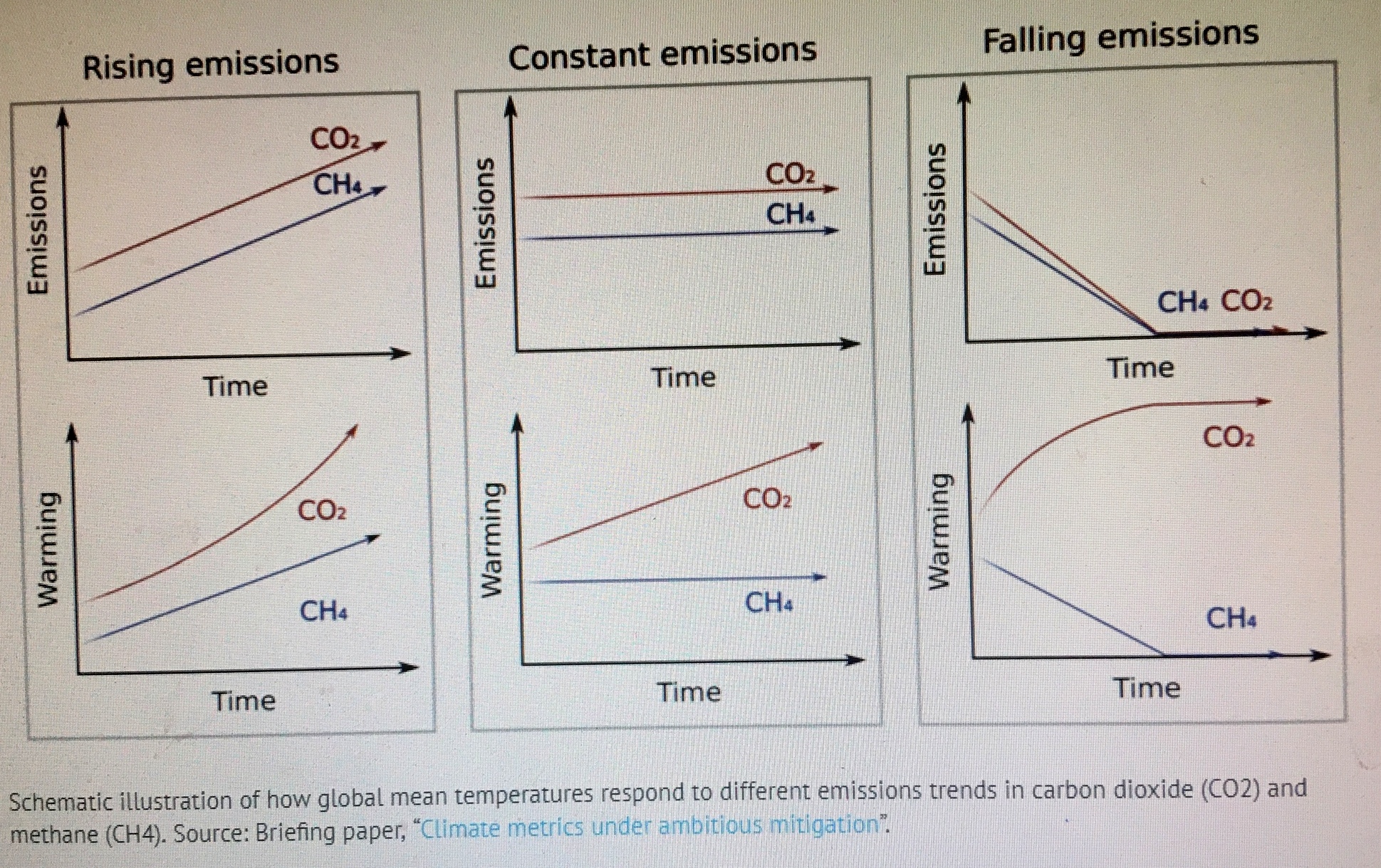
Schematic illustration of how global mean temperatures respond to different emissions trends in carbon dioxide (CO2) and methane (CH4) source Allen, Cain Lynch Frame (2018)
Summary The atmosphere, a major sector of the carbon cycle, manages methane (CH4) and carbon dioxide (CO2) very differently. Use of a Global Warming Potential ratio (GWP) to compare the future heating effect of CH4 emissions to that of CO2 emissions ignores those differences. In future scenarios where CH4 emissions have been level or falling steadily for ten to twenty years, CO2-e reckoned by GWP will predict huge ongoing additions by methane to heat-trapping. Actually in these scenarios there will be no further additions if the hypothetical trend holds. Methane emissions will equate to zero or even negative CO2-e. In contrast, CO2 emissions will keep adding to heat-trapping until they decline to net zero. Using CO2-e for methane hides the fact that reducing CH4 emissions instead of letting them rise would make an enormous improvement in the planet’s 2030 budget of heat-trapping GHGs. Banning new natural gas fracking wells would end the uptrend in gas production that underlies imputed uptrends in methane emissions.
The illustration above caught my eye a few months ago for its graphic challenge to the received wisdom that the global warming effect of methane (CH4) emissions over time is well-captured by a constant ratio (GWP) that compares their future warming effect to that of carbon dioxide (CO2) emitted at the same time. The comparison is expressed as CO2 equivalent or CO2-e.
In the bottom row above, CH4 heating effect does not parallel CO2 heating effect at all times as it should if they are related by GWP. Divergence between the CH4 and CO2 curves in the bottom row (warming vs time) is especially striking in the middle and right-hand panels. If emissions of both gases have been unchanged (middle column) for ten to twenty years, methane emissions at the same rate thereafter equate to the emission of no CO2. If emissions of both gases have been falling for ten years and keep to that trend (right-hand column), future methane emissions will permit atmospheric cooling even though future falling CO2 emissions will add to heating until they are nil.
The middle and right-hand columns represent “scenarios of ambitious mitigation.” These look today like fantasies, yet the (even more challenging) right-hand column must be realized if the living earth is to be recognizable in fifty years. The illustration shows a tremendous potential benefit to leveling out or (better yet) decreasing methane emissions that is missed completely by a GWP-mediated comparison to CO2 as CO2 equivalents or CO2-e Most enviro-activists don’t see this opportunity, especially re annual increases in withdrawals of natural gas that almost certainly cause increases in methane emissions.
CH4 methane
CO2 carbon dioxide
CO2-e CO2 equivalent, derived from GWP, of the heat-trapping capacity of a GHG emission, In this paper, methane is the only non-CO2 GHG considered.
CO2-e* CO2 equivalent of the heat-trapping capacity of a methane emission derived using GWP* Spoken of as “CO2-e star”
GHG Greenhouse gas
GWP Global warming potential of a GHG relative to CO2 over a specified time span
GWP* Variant metric to estimate future heating effect of a “short- lived” GHG or other climate pollutant relative to CO2 spoken of as “GWP star”
Mmt million metric tons, typically used for CO2
Tg million metric tons, typically used for methane
This paper aims to alert activists to how much leverage there is for mitigating global heating by getting methane emissions on a level plane or declining year-on-year for a decade or more. We are used to GWP as the metric for comparing the heat-trapping capacity of methane to that of CO2 over a specified time horizon, such as a hundred years. The conventional GWP says that an emission of methane will add to atmospheric heat-trapping in strict ratio to a like amount of CO2 emitted at the same time, the ratio being the chosen value of GWP.
A different usage of GWP, designated GWP* or “GWP star” by the multi-national group that advocates it, takes into account (as GWP does not) the difference in how the atmosphere manages CO2 and CH4 to create the models in the illustration above. In a 2018 paper members of the group wrote “Expressing mitigation efforts in terms of their impact on future cumulative emissions aggregated using GWP* would relate them directly to contributions to future warming, better informing both burden-sharing discussions and long-term policies and measures in pursuit of ambitious global temperature goals .”[emphasis added]
Sidebar on GWP: Values for GWP on a 100-year horizon in recent use range from 25 to 34, with no consensus. The current GWP for a 20-year horizon (GWP20) is 86. Authorities disagree on which horizon to use. Ocko et al [Science 5 May 2017] suggest a dual metric called GWP100/20 , analogous to mpg hiway/city. I am convinced that GWP20 is more correct for considering the next twenty years; this paper, however, will use only a GWP100, with value 28. That is the GWP used by the multi-national group that has proposed the alternative metric GWP* explored in this paper
Conventional GWP usage predicts that (say) 300 Tg (= 300 million metric tons or Mmt) of methane emitted in (say) 2030 will increase atmospheric heat-trapping during the following ten years as much as will 8400 Mmt of CO2 emitted in the same year. This appalling prospect is not necessarily correct. Actually, how much a future methane release will add to atmospheric heat-trapping will not on its size but on the rate of change in annual methane emissions over the previous ten to twenty years. With CO2, by contrast, all future emissions add to the atmospheric burden regardless of the trend in annual emissions over preceding years. The difference is crucial in thinking about the utilities of curbing methane emissions over the next two decades..
Suppose that 2019 human-influenced methane emissions are 300 Tg (a figure plucked from the air). We want to estimate in 2019 the effect of methane releases during 2029 on global surface temperature over the following ten to twenty years. The motive is to decide how much benefit in temperature moderation can be got from keeping annual releases 2019-2029 at or below 300 Tg Applying a GWP100 to 300 Tg of emissions in 2029 yields the monstrous CO2 equivalent above, 8400 Mmt. Seeing how the atmosphere handles methane as opposed to CO2, however, offers a revelation that will surprise many well-informed people. If (big if) annual methane emissions have been uniformly at or below 300 Tg/yr from 2020 through 2029, the release of 300 Tg in that last year will add to atmospheric heat-trapping capacity the equivalent of zero (0) Mmt CO2. Methane releases 2020-2028 will have added a great deal to heat-trapping capacity that obtained in 2019, but releases of the same or smaller size in 2029 and the years to follow will not add any more. Put another way, CO2-e* = 0.
That observation may seem wishful thinking, because the world is hardly on course to hold methane emissions in the next 10-20 at or below current levels; the very opposite is true. Nonetheless, it is conceivable that public pressure + resistance could end the annual growth of gas extraction, thereby curbing methane emissions over the next decade.
The point here is that when thinking about methane for a ten-twenty year future GWP and the related CO2-e are not apt metrics. My quest to spread the word on why GWP* and the associated CO2-e* spotlight the benefits of “ambitious mitigation” led me to a graphic explanation. It begins with a narrative comparing the careers of methane molecules and CO2 molecules in the atmosphere.
Most methane molecules in the atmosphere have by ten years after entrance been changed into CO2 through a series of chemical reactions in the oxidizing “atmospheric methane sink.” If each of these molecules is not replaced with another from a human-influenced source, the atmospheric inventory of methane will begin to decline toward the level set by “natural” (not human-influenced) methane releases. An individual methane molecule survives only a few years. A one-time bolus of methane molecules without replacement will have dwindled to almost none within roughly ten years. Methane is “short-lived.”
Most CO2 molecules that arrived at the same time as the methane ones have also left the atmosphere in those ten years to return to earth. They departed, however, as CO2, not yet transformed into another chemical as will happen once they cycle back to earth or ocean. On the earth’s surface the carbon atom drops its attached oxygen atoms to become part of (e.g.) a plant sugar. Eventually via respiration or decomposition the typical one will hook up with two new oxygen atoms as CO2 and be airborne again.
Each CO2 molecule as it leaves the atmosphere is quickly replaced by another CO2 in the teeming carbon cycle. That cycle eagerly takes up CO2 from plant and animal respiration and surface ocean water. It also pulls in carbon that has been out of the atmosphere and now re–enters it as CO2 after years (e.g. young trees pulped or burnt); centuries (e.g. old growth pulped or burnt or decaying; untouched prairie soils tilled, ag soils washed-out ); or geological eras (e.g. fossil fuels extracted and burned, cement made from limestone). Much of this re-entry, not all, is human-influenced. Human-influenced CO2 emissions, however, are a small part of the carbon cycle inventory, whereas human-influenced CH4 emissions make up much of the associated atmospheric methane cycle. Thus inventory of CO2 molecules in the atmosphere cannot decline unless carbon is sequestered at higher rates than now prevail. The inventory is long-lived; individual CO2 molecules are not. It is misleading that CO2 is called “long-lived.”
In a banking analogy, methane is a busy checking account with cash flow: deposits, withdrawals and fluctuating daily balance. CO2 is a savings account whose manager replaces every withdrawal the same day and makes deposits to boot, building up the stock. Thus methane is termed a “flow gas” and CO2 a “stock gas.”
Four scenarios of emission rates for CO2 and methane are presented below in simple graphs. Each starts with an imaginary burst or “pulse” of 1000 arbitrary mass units of the gas released on December 31, 2020 into an atmosphere until then devoid of that gas. What becomes of the molecules in that release in the next fourteen years in each scenario is plotted in a pair of graphs, with methane first (white background), then CO2 ( black background). All data are hypothetical, for illustrative purposes.
Graph Pair Emissions Scenario
{1 and 2} nil no human-influenced emissions
{3 and 4} no change year on year level plane
{5 and 6} down 20 units/yr over 14 yrs falling
{7 and 8} up 20 units/yr over 14 yrs rising
In scenario 1 no more gas is emitted after the one pulse. On Dec 31, 2020 the methane inventory (= count or “census count”) is 1000 units. At the end of 2021, those 1000 units have been reduced to 900 by chemical reactions in the atmospheric sink. At the close of 2022, the “census count” is down to 800. With an average of 100 units disappearing each year, the original group ( = “cohort”) is at nil by 2030. This outcome is shown in Graph 1. The life span of a one-off pulse emission of methane in this example is ten years; the survival time of a single molecule averages roughly 5 years. Note well: The actual life span of a pulse emission of methane cannot be measured; it is not exactly ten years, but somewhere between eight and twelve.
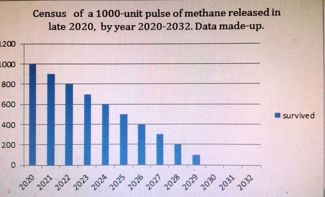
Graph 1. “no emissions” Year-end census count of a 1000-unit pulse of methane released in late 2020 with no emissions thereafter, by year, 2020-2032. Data are made-up. Plot is schematic
The CO2 story is altogether different. Imagine a pulse of 1000 units CO2 emitted December 31, 2020, with no more after that. Every CO2 molecule in this pulse that leaves the atmosphere for a different sector of the carbon cycle (e.g. plants, ocean) gets replaced by another in that cycle almost immediately; so, the census count does not go down. Maybe a quarter of the molecules in the original population have moved on in the cycle after a year. Each, however, has figuratively “signed out” to an incoming CO2 that will probably itself swap places with yet another in a couple of years. After ten years, most of the CO2s in the 2020 pulse are no longer aloft, but each has been replaced with another CO2, and the replacement perhaps replaced. The atmospheric residence time of a single molecule in the original pulse is only three to four years, but because of the capacity and robustness of the earth’s carbon cycle, the concentration impact of the hypothetical 1000 units/yr of CO2 emitted even ten years earlier will remain at 1000 units for centuries. Graph 2
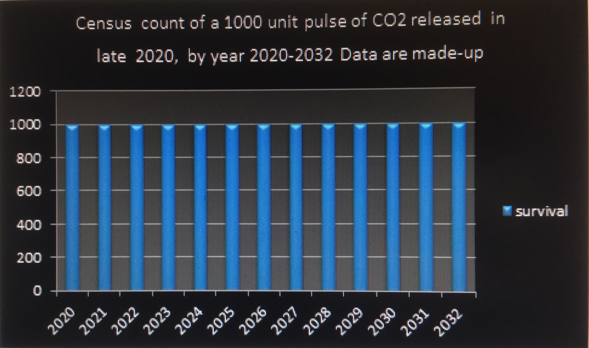
Graph 2. “no emissions” Year-end census count of a 1000-unit pulse of CO2 released in late 2020 with no emissions thereafter, by year, 2020-2032 Data made-up Plot is schematic
The two scenarios above allowed for no emissions after the initial pulse. What happens if there are subsequent emissions?
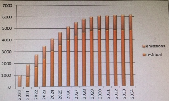
Scenario 2, with emissions on a level pace for all years, appears in the next two graphs. In graph 3 below, methane emissions are 1000 units/yr. To make the model as simple as possible, 100% of the methane emissions in a calendar year remain in the atmosphere throughout that year, then begin to be cleared roughly stepwise so that all are gone by ten years after emission. [Ten years is an arbitrary number; using eight or twelve would change the inflection point of the inventory growth curve but not its ultimately attaining zero slope.] At year’s end 2020 the burden is 1000. Emissions in 2021, added to what carried over from 2020, a portion of which was “scrubbed” in 2021 (chemically transformed into something other than methane), raise the burden (“inventory”) to 1900.
At the end of 2022 the inventory is the sum of residual from the 2020 emission (now reduced to 800 units) + residual from the 2021 emission, now down to 900 units + the 1000 units emitted in 2022. Each year after that for a few years the inventory increases. Methane accumulates in the atmosphere until (in this hypothetical example) 2029. In that year, due to their short atmospheric lifetime, methane molecules vanish at the same rate at which new ones come in with emissions. After 2029, therefore, the annual emissions, steady at 1000 units/yr, no longer add to the methane burden (5500 units CH4) that characterizes any given subsequent year. They do sustain it at that monstrously high level, 4500 units above the baseline of 2020. After 2029, CO2-e* = 0
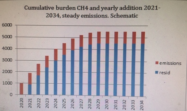
Graph 3. “level plane” Cumulative burden of atmospheric methane (sum of blue and red) following a 1000 unit pulse Jan 1 2020, by year and component (residual or annual emission) 2021-2034. Yearly emissions are constant-value Graph is schematic. Data are made-up. Vertical axis does not refer to any specific physical unit.
Compare the methane graphic story above with that of CO2 below in Graph 4. With constant annual emissions of 1000 units preceding 2034, the addition in 2032 to the inventory of the previous year is 1000 units. The cumulative addition to the 2020 burden of 1000 units CO2 by the end of 2034 is 14000 units CO2 .
Attention! In this imaginary scenario of level-plane emissions for each gas beginning 2020, the CO2 burden in 2034 is 14,000 units above the 2020 baseline; the methane burden has gained less, 4500 units. Whatever horizon GWP one uses, however, the 4500 unit addition to total atmospheric heat-trapping capacity due to methane in these years is enormously more than that due to an added 14000 units of CO2 . At the least the former is equivalent to 4500 * 25 = 112,500 units CO2-e ; at the worst, to 4500 * 104 = 468,000 units CO2-e .
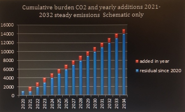 Graph 4. “level plane” Cumulative burden of atmospheric CO2 (sum of blue and red) by year and component (residual or annual emission) 2021-2034. Yearly emissions are constant value. Graph is schematic. Data are made-up. Vertical axis does not refer to any specific physical unit.
Sidebar Obviously, these four graphs do not accurately represent reality.
- No precise count of units or molecules is possible,
- Any count of surviving methane units, if possible, would not change in so neatly stepwise a manner, nor would emissions of either gas be just the same year to year.
- The atmospheric inventory of either gas of course pre-existed the imaginary 2020 pulse emission and was much larger.
- Setting the early-2020 inventory counterfactually at nil in this model makes the annual changes depicted relatively more prominent. Still, the plot for each gas of the yearly census of its 2020 pulse emission over ten years represents well the survival curve of the relevant census for each gas whether we start with a zero inventory on Dec 31 2020 or a real inventory of Tg or Mmt.
- Saying emissions of each gas are 1000 units/yr to start makes it seem that the tonnage of emissions yearly is the same for CO2 and CH4 where in reality the mass of CO2 emitted is more than one hundred times that of CH4.
None of these simplifications, though, exaggerates the central message of this ultra-simplified model: in this scenario of emission rates unchanged for ten years to 2029 and beyond, with methane there is no addition after 2029 to the inventory of that year though it is by then is 450% of the baseline. For CO2 in the same scenario there is a substantial yearly increment to the previous year’s inventory.
Whether or not there is arithmetic net addition is extremely important. The customary way to rate the effect on atmospheric heat-trapping of a future methane emission is to multiply the mass emitted by a GWP. Some people use GWP20 of 86; others a GWP100 for which values of 25, 28 and 32 are all current. Applying a GWP100 to 1000 units of methane emitted in 2030 in the Graph 3 scenario would have that amount adding to the atmosphere over the subsequent ten years as much heat-trapping capacity as 28000 units of CO2 emitted in 2030. On the contrary, those 1000 units of methane emitted in this scenario would actually add nothing to the then-current atmospheric heat-trapping capacity. They are equivalent in that sense to the addition of zero units of CO2, not 28000.
This is not to say that methane will not continue to harm life on earth if emissions of it can ever be held steady for a decade. The graphs above make clear that ten upcoming years of steady emissions will add enormously to the atmospheric heat-trapping capacity we suffer in 2019. Only when those ten years or so are history will continued emissions at the same or lower level stop adding. It is to say that methane is an exception to the prevailing idea that all GHG emissions in all scenarios are additions to inventory, as is the case with CO2, and can be duly assessed with GWP.
The third scenario imagines slowly-falling emissions of each gas. Graph 5 plots methane emissions being lower stepwise by 2% (20 units) of baseline per year The total burden peaks in 2028, to drop slightly thereafter even though emissions are still substantial. Methane keeps contributing to total heat-trapping. Far from adding to it, however, it sets the stage for a little relative cooling. The pace of emissions after 2028 is too slow to replace all the methane molecules that vanish each year after that . In this scenario, someone wedded to GWP would say that methane emissions in 2034 (imagined as 720 units) are equivalent to 720 * 28 = 20160 units of CO2. As additions to then-prevailing heat-trapping capacity, they are equivalent to 0 units of CO2. Repeat: they are sustaining heat-trapping but not as strongly as do level-plane emissions They do not add to it. They permit some cooling by being inadequate reinforcements for the earlier cohorts. After 2029 CO2-e* has a negative value; CO2-e* < 0
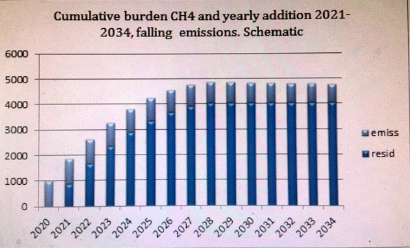
Graph 5. “slow fall” Cumulative methane burden with falling yearly additions after a 1000 unit pulse emission in early 2020, by year 2020-2032. Data are made-up. Graph is schematic.
The comparable slow fall scenario for CO2 is shown in Graph 6, in which annual emissions are 1000 units in 2021. They are reduced thereafter by the same annual decrement, averaging 2%/ of baseline per year, as for methane in Graph 5. By 2034 , 13,600 units have been added to the 2020 baseline.
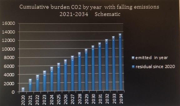
Graph 6. “slow fall” Cumulative CO2 burden with decreasing yearly additions after a 1000 unit pulse emission in early 2020, by year 2020-2032. Data are made-up. Graph is schematic.
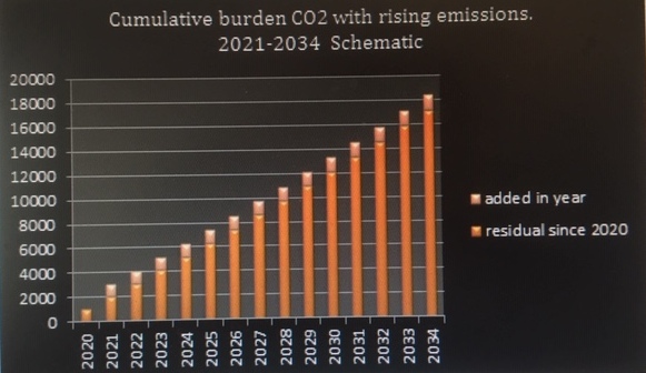
The fourth scenario is rising emissions of both gases Looking at predictions of increasing natural gas production for the next twenty years, it is folly not to fear that methane emissions due to losses from the supply chain will rise concomitantly. Graph 7 presents a scenario in which methane emissions go up on an average of 2 % of baseline (20 units) per year. [This rate should not really be considered “slow.”] In 2034 emissions are (made-up data) 1280 units, higher than the baseline of 1000 units and higher than 1260 the previous year. Strict GWP100 protocol would tag the 1280 units emitted in 2034 as 35840 units CO2-e.
The GWP* method could be used to reckon units of CO2-e* using the 100 year horizon recommended for GWP* by Allen et al: There was an increase of 280 units over 14 years; hence 280 units * 28 * 100 yrs/14 yrs = 56000 units CO2-e*. [After I had drafted this blog, a new paper by the same group appeared (Cain, Allen et al 2019). The authors prefer to CO2-e* a new comparison metric called CO2-we for “warming equivalent.” The CO2-we for these hypothetical data is 49,000 Mmt.] Both are higher than the CO2-e.
That CO2-e* computed with GWP* is greater than CO2-e computed with GWP100 brings out another splay between GWP and GWP* as metrics to compare methane and CO2. If annual emissions are rising, higher rate of change makes the value of CO2-e* exceed that of CO2-e. If the hypothetical data set here is revised to make methane emissions in 2034 be 1100 units, only 100 units higher than fourteen years before instead of 280 units , the CO2-e would be 30800 units and the CO2-e* found with GWP* would be less, 20000 units. [The CO2-we is 22000 Mmt. ] For this much slower ( + 0.7%) increase in annual emissions, C02-e > CO2-we > CO2-e*.
Aside: How to calculate CO2-e* and CO2-we in present-day scenarios of rising methane emissions is discussed in a different blog. It is important. Today’s blog focuses more on desirable, and not impossible, scenarios of ambitious mitigation illuminated by the GWP* method.
Graph 7. “rising” Cumulative methane burden with increasing yearly emissions after a 1000 unit pulse emission in early 2020, by year 2020-2032. Data are made-up. Graph is schematic.
In Graph 8 below, the lineup of annual increases for CO2 emissions ( + 20 units/yr) is the same as that for methane emissions in Graph 7. Result: In 2032, the cumulative burden of CO2 is 14,444 units 13,444 units above the 2020 baseline.
Graph 8. “rising” Cumulative CO2 burden with increasing yearly emissions after a 1000 unit pulse emission in early 2020, by year 2020-2032. Data are made-up. Graph is schematic.
Table 1 below summarizes the four scenarios. Scenario 1 (no emissions after 2020) is literally impossible, purely illustrative. Among all other three scenarios, fourteen years of methane emissions have added considerably as of 2034 to the methane inventory of 2020. All the same, in “ambitious mitigation” scenarios 2 and 3 (level and falling emissions, respectively), emissions after 2029 no longer add to the previous year’s inventory. This runs counter to the prevailing arithmetic of greenhouse gases, that emissions always add to the atmospheric inventory of that gas and that the heating effect of the addition can be compared to that of CO2 by a factor of GWP100 or GWP20.
No one will be surprised that when emissions of methane rise steadily for years this gas will add to heat-trapping capacity of the atmosphere. What might seem surprising is that very small annual increases sustained over a decade do not cause as large an increment to the heat-trapping capacity of the previous year’s methane burden as would be predicted applying a GWP to the year’s methane emissions. CO2-e* < CO2-e in this narrow range of suboptimal mitigation. For this ability to buffer partially against small increments, life on earth is indebted to the methane sink, a wondrous phenomenon outside the ken of most people.
|
Scen- |
Emiss |
CH4 in |
CO2 in |
CH4 in |
CO2 in |
change in |
change in |
change in |
change in |
|
ario |
2021 to |
2020 |
2020 |
2034 |
2034 |
CH4 2020 |
CO2 2020 |
CH4 2033 |
CO2 2033 |
|
2034 |
to 2034 |
to 2034 |
to 2034 |
to 2034 |
|||||
|
1 |
nil |
1000 |
1000 |
0 |
1000 |
-1000 |
0 |
0 |
0 |
|
2 |
level |
1000 |
1000 |
5500 |
15000 |
4500 |
14000 |
0 |
1000 |
|
3 |
falling |
1000 |
1000 |
4770 |
13620 |
3770 |
12620 |
-20 |
700 |
|
4 |
rising |
1000 |
1000 |
6190 |
18380 |
5190 |
17380 |
20 |
1700 |
Table 1. Comparisons over time between CH4 and CO2 in raw tonnage, across the four scenarios
In summary, when the rate of change in emissions of methane has been zero or negative for ten years, future emissions holding to that trend do put methane into the atmosphere. They do not, however, add to the inventory of the year before. When the rate of change has been positive, future emissions of methane do add to the most recent inventory. With CO2, in contrast, all future emissions add to the cumulative CO2 inventory. This makes comparisons between the heat-trapping effects of methane and CO2 that use GWP deceptive, especially in scenarios of ambitious mitigation of methane like numbers 2 and 3 above.
Discussion Since the world is unlikely to achieve ambitious mitigation of methane, does it really matter that GWP misrepresents the comparison with CO2? Definitely yes. It is theoretically possible that the world could go soon into a decade in which methane emissions do not rise year on year, even decline. Ending the growth of unconventional natural gas withdrawal or “fracking” would very likely end the growth of annual methane emissions imputed from rising atmospheric level of the gas. To achieve such an end to growth it is not necessary to “ban fracking;” that horse is out of the barn. It is necessary to ban all new fracking wells; that is a horse of a different color.
Industry says the lifespan of a fracking well is twenty to forty years. The economically remunerative life is much shorter, perhaps six years on the average. Gigantic forces of big business that manipulate governmental policy and try to bend public opinion oppose a ban on new wells. There are strong headwinds against a ban on new fracking wells, as strong as those against (say) new arms treaties or restrictions on firearms. There are also portents, though, that clean energy can soon undercut natural gas. The fight against new fracking is worth all the effort we can give it and more.
Using only a conventional GWP to assess the outcome circa 2030 of curbing of methane emissions starting 2020 hides the enormous benefits in the future of the redirection that stand out in the table above. We must redirect to save our living earth and we should use the science behind GWP* to guide us.
Appendix The major human-influenced emissions of methane are, approximately in this order most to least: losses during extraction/withdrawal and distribution of fossil fuels; methane from ruminant animals as eructation and in manure; landfills and sewage disposal; paddy rice growing; and burning of biomass. Major human-influenced emissions of CO2 are combustion of fossil fuels and cement manufacturing.
Background reading besides the hyperlinks
Myles R. Allen, Keith Shine et al “A Solution to the Misrepresentation of CO2-equivalent emissions of short-lived climate pollutants under ambitious mitigation” https://www.nature.com/ articles/s41612-018-0026-8
Cain, Lynch, Allen et al Improved calculation of warming-equivalent emissions for short-lived climate pollutants. npjClimate and Atmospheric Science 2 (Sept 4 2019)
https://www.oxfordmartin.ox.ac.uk/downloads/briefings/Short_Lived_Promise.pdf Myles Allen 2015
http://www.skepticalscience.com/co2-residence-time.htm
https://www.anchorageromneys.com/2019/06/over-heaters-anonymousthe-methane-diet/
Allen, Fuglestvedt, Shine et al . New Use of Global Warming Potentials to Compare Cumulative and Short-lived Climate Pollutants. Nat Clim Change 6:773-776 2016
Acknowledgments: I thank for their gracious help in my self-education on methane the following scientists: Michelle Cain, Oxford Martin School, University of Oxford; Ruth DeFries, Columbia University; Steven Hamburg, Environmental Defense Fund; Robert Howarth, Cornell University; John Lynch, Food Climate Research Network University of Oxford; Frank Mitloehner, UC Davis; Bryce Payne, Jr., Wilkes University and Gas Safety, Inc; Sara Place, National Cattlemen’s Beef Association; Jeanne Stellman, Columbia University; Evelyn Wright, Sustainable Energy Economics, Kingston NY. Thanking them does not imply their endorsement. I am responsible for any errors of fact or interpretation. All opinions expressed are my own.
Stephen Q. Shafer MD MPH MA Saugerties NY sqs1@columbia.edu 917 453 7371
Permission granted to reproduce the above work in whole or part with the permalink cited http://www.anchorageromneys.com/2019/10/co2-e-is-the-wrong-metric-for-methanes-heating-effects/